

Why Data Formats Matter More Than You Think
Most data engineers have heard of Parquet, ORC, or Arrow. These formats underpin the modern data stack — from Spark and Snowflake to BigQuery and Redshift Spectrum. But while they’re everywhere, many teams treat them as black boxes: pick a format, save the file, move on.
Yet the internal mechanics of these formats matter. Columnar layouts, compression schemes, encoding strategies, and schema evolution rules can directly impact:
query performance
cost of storage and scanning
compatibility between engines
correctness in long-running pipelines
A deep understanding of how data formats behave under the hood — how they store information, how metadata flows through pipelines, and how various engines interact with structure and compression — is key to making informed architectural decisions, optimizing runtime behavior, and avoiding subtle bugs across systems.
Row vs Column Storage: The Foundational Tradeoff
Data can be stored either row by row or column by column, and this structural decision has deep consequences for performance, compression, and use cases.
In row-based formats, like JSON, CSV, and Avro, all fields of a record are stored together. This layout is ideal for:
write-once, read-whole workloads (e.g. log ingestion)
transactional systems where individual records are frequently updated or retrieved
streaming pipelines, where each message is self-contained
However, row-oriented storage becomes inefficient when only a subset of fields is needed — a common case in analytics. Reading millions of rows just to extract a few columns leads to wasted I/O and CPU.
Columnar formats, such as Parquet and ORC, invert the structure: all values of a single column are stored together, often across large batches of rows. This layout enables:
predicate pushdown: reading only the necessary columns
vectorized processing: CPU-friendly access patterns
high compression ratios: due to similar adjacent values
The tradeoff is write complexity. Appending new rows requires buffering data across all columns. Random access to individual records becomes expensive. Columnar formats favor append-heavy, read-optimized workloads — particularly for OLAP, machine learning, and data lake use cases.
Some formats, like Apache Arrow, push this model further by representing columns as in-memory vectors, aligning with SIMD instructions and GPU pipelines.
Choosing between row and column layout is not just about file format — it reflects the workload itself. The right structure accelerates queries, reduces costs, and shapes how tools interact with the data beneath.
Parquet: The Workhorse of Analytics
Parquet is a binary, columnar format designed for efficient analytical workloads. Its internal layout is optimized for parallel reads, filter pushdown, compression, and nested schemas.
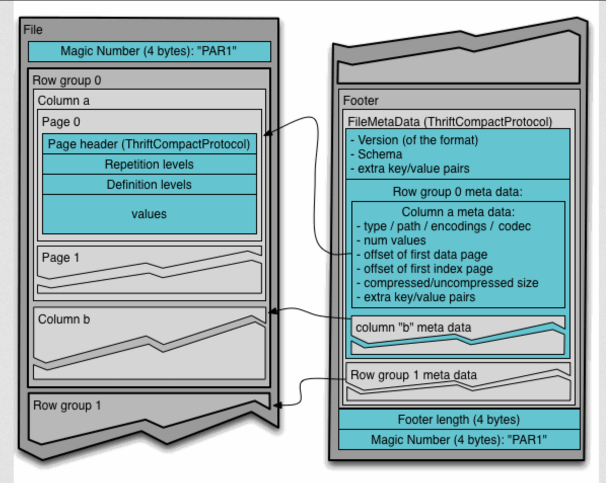
A Parquet file consists of three parts:
Header: a 4-byte magic number (
PAR1) identifying the format.Data Blocks (Row Groups): horizontal partitions of rows, where data is stored column by column.
Footer: contains metadata — schema, column types, encodings, statistics, and physical offsets — and ends with
PAR1to support reverse scanning.
Row Groups and Column Chunks
Row groups are self-contained blocks (typically 64–512MB) that can be read in parallel. Each contains column chunks, storing all values for a single column. This layout enables true columnar access and efficient filtering.
Within each column chunk, data is split into pages, the smallest I/O unit:
Row Group 1
├── Column Chunk: user_id
│   ├── Page 1
│   ├── Page 2
├── Column Chunk: event_type
│   ├── Page 1
│   ├── Page 2
Page types include:
Data Pages: encoded values + definition/repetition levels
Dictionary Pages (optional): if dictionary encoding is used
Each page starts with a Thrift-encoded header describing its type, encoding, value count, and sizes (compressed/uncompressed).
Inside a Data Page
A Data Page contains:
Repetition levels (for nested types)
Definition levels (null tracking)
Encoded values (dictionary, RLE, or plain)
For example, a nullable int32 column would store:
A compact bit-packed stream of definition levels (0 = null)
Followed by encoded integers
Modern engines like Spark or DuckDB read pages lazily and skip them entirely when predicate filters rule them out.
Page Size and Performance
Page size significantly impacts performance. Smaller pages allow finer-grained filtering but incur more overhead. Larger pages are more efficient for I/O but can hurt memory usage and pruning accuracy.
Typical page sizes range from 8 KB to 1 MB, and most engines allow tuning this during write time.
Encoding, Compression, and Schema Design
Parquet leverages its columnar structure to apply powerful encoding and compression techniques that reduce file size and accelerate scans. These optimizations operate at the page level, enabling independent decoding and selective skipping.
Encoding Techniques
Each column can use a tailored encoding based on its type and value distribution. Common methods include:
Plain Encoding – raw values stored directly; simple but inefficient for repetitive data.
Dictionary Encoding – values mapped to indexes via a dictionary page; ideal for low-cardinality strings or enums. Not used when cardinality exceeds ~65,000.
Run-Length Encoding (RLE) – compresses repeated sequences (e.g.
1,1,1 → [1×3]); also used for null markers.Delta Encoding – stores differences between consecutive values; useful for timestamps or sorted integers.
Bit-Packing – tightly encodes small fixed-width integers (e.g. booleans, enums).
Byte Stream Split – separates bytes of floating-point values to improve compression (used in newer Spark/Arrow versions).
Parquet may mix encoding types:
Across columns (e.g., strings with dictionary, integers with delta)
Across row groups or even pages within a column
This flexibility improves performance but increases decoder complexity.
Compression Codecs
After encoding, Parquet applies optional compression to each page. Common codecs:
Snappy (default) – fast and lightweight.
Gzip – stronger compression, but CPU-intensive.
ZSTD – modern balance between speed and compression ratio.
Others: LZO, Brotli, LZ4 — supported in some engines.
Since compression comes after encoding, efficient encodings amplify overall savings.
Schema and Nested Types
Parquet supports flat and nested data using a typed tree schema, serialized in the footer using Thrift. Fields include:
Primitive types:
int32,binary,boolean, etc.Logical types:
UTF8,DECIMAL,TIMESTAMP, etc.Repetition modifiers:
required– always present,optional– may be null,repeated– used for lists.
Example schema:
message UserEvent {
  required int64 user_id;
  optional group metadata {
    optional binary country (UTF8);
    optional binary device_type (UTF8);
  }
  repeated group clicks {
    required int64 timestamp;
    optional binary url (UTF8);
  }
}
This defines:
A required scalar field,
An optional nested struct,
A repeated group (list of clicks).
Definition and Repetition Levels
To encode nullability and nested structure efficiently, Parquet introduces:
Definition Level (DL) – how many optional fields are defined along a path (e.g., null URL inside a defined click → lower DL).
Repetition Level (RL) – depth within a repeated field; used to reconstruct list boundaries.
These levels are stored alongside values using RLE or bit-packing. They allow full reconstruction of complex structures without explicit nulls or padding.
Schema Evolution
Parquet supports limited forward evolution:
Safe: adding new
optionalfields (appear as nulls in old data)Unsafe: renaming fields, changing types, or reordering
Engines read the footer schema and try to align fields at runtime. Spark and Arrow tend to be forgiving; Hive is stricter.
Metadata, Predicate Pushdown, and Read Optimization
Parquet’s layout allows engines to skip entire blocks of data without reading or decompressing them — based on filter conditions and column usage. This is achieved via columnar storage, file-level metadata, and statistics stored in the footer.
Row Group Statistics and Skipping
Each row group contains min/max values per column, null counts, and physical offsets. At query time, engines (e.g., Spark, Trino, DuckDB) inspect this metadata to skip irrelevant data.
Example:
Query: WHERE country = 'DE'
Row group min/max: 'US' → 'US'
⟶ The group is skipped — no need to scan.
Columnar storage also enables column pruning:
SELECT user_id reads only the relevant column, skipping all others.
These optimizations reduce I/O, CPU usage, and cost — especially in systems like BigQuery or Athena.
Footer Layout and Role
The footer acts as an index, storing:
Schema definition (via Thrift)
Row group metadata: offsets, encodings, statistics
Column-level compression and page structure
It is located at the end of the file:
[ ... data blocks ... ][ metadata ][ footer length ][ magic: PAR1 ]
Readers scan the last few bytes to locate and parse the footer, avoiding a full file read.
Newer versions support page-level indexes and Bloom filters, allowing fine-grained skipping — although support varies by engine.
Best Practices
To ensure performance and compatibility:
Row group size: 128–512MB is ideal.
Small groups increase metadata overhead, large ones hurt parallelism.Compression: Use Snappy for speed, ZSTD for better ratios.
Avoid Gzip unless storage cost is critical.Dictionary encoding: Enable for low-cardinality columns (e.g. countries, enums).
Avoid on high-cardinality fields.Avoid small files: Engines like Spark or Trino perform poorly with many small files.
Use batch writes or compaction.Flatten nested schemas: Deeply recursive structures increase decoding cost and reduce scan efficiency.
Validate schema evolution: Adding new optional fields is safe.
Renaming or type changes often cause compatibility issues.
Common Pitfalls to Avoid
Disabling statistics or writing uninformative types (e.g. binary for everything)
→ disables predicate pushdown.Using inconsistent nulls or deeply nested optional fields
→ leads to poor compression and broken filters.Writing many small row groups or mismatched schema versions
→ bloats metadata and breaks reads.
Ecosystem Tools
Use tools like:
parquet-toolsfor structure inspectionDuckDB and Apache Arrow for fast analysis and validation
PyArrow/Spark for full-featured, metadata-rich writes
ORC: Columnar Format with Built-in Indexing
ORC (Optimized Row Columnar) was designed as a high-performance storage format for Hadoop workloads, originally by Facebook and Hortonworks. Unlike general-purpose formats like Parquet, ORC was purpose-built for batch analytics, tightly coupled with Hive and optimized for high-throughput reads and filter-heavy scans.
Stripe-Based Layout and Embedded Metadata
An ORC file is organized into stripes, each typically holding between 250,000 and 1 million rows. Every stripe contains three main components: index streams (lightweight statistics and null flags), data streams (the encoded column values), and a stripe footer with metadata.
This localized metadata structure allows ORC to bypass the global file footer for many operations. Readers can apply filters and plan execution using only the stripe-level information — significantly improving scan performance in distributed environments.
Fine-Grained Indexing
One of ORC’s most distinctive features is its built-in row indexes. These are written at fixed row intervals (e.g., every 10,000 rows) for each column and include:
Minimum and maximum values
Null presence flags
Byte offsets to row positions
This allows engines to skip parts of a stripe based on query filters — something Parquet cannot do without reading its full footer.
Optimized Encoding and Compression
ORC tightly integrates encoding decisions with indexing and compression. Each column stream within a stripe is encoded using the most efficient strategy for its type and distribution:
Dictionary encoding for low-cardinality strings, with automatic fallback to direct encoding
Delta encoding for sorted numeric fields like timestamps
Boolean RLE for compact encoding of binary values
Zigzag + XOR compression for floating-point values
Once encoded, data is compressed using codecs such as ZSTD (the default in most engines), Snappy, or Zlib. ORC also compresses its metadata — including indexes and footers — providing efficiency advantages for remote reads in object stores.
Strong Typing and Nested Structures
ORC enforces strong typing with explicit support for:
Timestamps with nanosecond precision
Decimals with controlled precision and scale
CHAR/VARCHAR types with length constraints
Nested structures, including lists, maps, and structs
Unlike Parquet, which annotates logical types separately, ORC embeds type definitions directly into its schema, improving validation and compatibility across query engines.
Practical Advantages in Query Engines
Thanks to its localized stripe footers, ORC enables faster metadata access during query planning. Engines like Hive, Trino, and Spark can read and scan stripes independently, apply pushdown filters without reading the full file, and parallelize access with minimal coordination.
This architecture is particularly advantageous in interactive or real-time scenarios — such as Hive LLAP — where quick predicate evaluation and scan planning are essential.
ORC File Footer, Indexing, and Practical Guidance
ORC files conclude with a compact, highly structured footer and a lightweight postscript block. This design enables efficient access patterns ideal for distributed storage systems like HDFS or Amazon S3.

Footer and Postscript Structure
Located near the end of the file, the footer contains:
The full schema, including nesting and types
Stripe locations and sizes
Optional global statistics per column
Custom metadata (e.g., writer versions or user-defined tags)
Immediately after the footer comes the postscript — a small (~16–32 bytes) block that stores:
Footer length
Compression settings
File version
Because the postscript is of fixed size, readers can jump directly to it, determine how to decode the footer, and begin reading stripes — all with minimal I/O. This is especially beneficial when scanning large datasets stored remotely.
Min/Max Statistics and Predicate Filtering
ORC maintains accurate, validated statistics at both file and stripe levels, including:
Minimum and maximum values per column
Null counts
Byte ranges for each column stream
These are leveraged for efficient filtering:
Stripe skipping based on filter conditions
Row group skipping via row-level index streams
Bloom filters for fields like user ID, country, or SKU — if enabled at write time
Unlike Parquet, ORC validates these statistics during file write, ensuring reliable filter pushdown in supported engines like Hive, Trino, and Spark.
Practical Guidelines for Effective ORC Usage
While ORC delivers excellent performance for batch analytics, optimal results depend on thoughtful usage patterns.
Stripe Sizing and File Layout
Aim for large stripes — typically 64MB to 256MB compressed. This strikes a balance between parallelism and metadata efficiency. Too many small stripes or files can:
Inflate overhead for readers
Reduce predicate filtering performance
Lead to fragmented and inefficient scans
Use engines that write in batches (e.g., Spark, Hive) and periodically compact files in streaming workflows.
Leverage Built-In Index Streams
Each stripe embeds row-level indexes for every column, enabling fine-grained filtering without reading the global footer. These include:
Min/max values
Presence (null) bits
Byte offsets
Design schemas with commonly filtered columns placed early and consider sorting on these fields to further enhance pruning.
Use Bloom Filters for High-Selectivity Columns
For filter-heavy columns (e.g., email, user_id), ORC supports optional Bloom filters. When enabled:
They help reject non-matching values quickly
Reduce decompression and I/O
Are compact and inexpensive to store
Enable them via engine-specific settings, such as orc.bloom.filter.columns in Hive or Spark.
Encoding and Compression Strategy
ORC automatically selects encodings based on column type and data distribution:
Dictionary for low-cardinality text
Delta for sorted numbers and timestamps
RLE and bit-packing for booleans and small integers
Compression options include ZSTD (default in modern setups), Snappy, and Zlib. ORC also compresses its metadata, reducing scan overhead in remote or large-scale deployments.
When ORC Fits — and When It Doesn’t
ORC is highly effective in:
Batch-based processing pipelines
Stacks using Hive, Trino, or Spark
Scenarios with sorted and partitioned datasets
Workloads with stable schemas and frequent filtering
However, it’s less ideal for:
Real-time ingestion or row-at-a-time updates
Lightweight or flexible workflows (e.g., Python/Pandas-based stacks)
Scenarios requiring frequent schema evolution or full interoperability
In essence, ORC is a strong fit for mature data lakes focused on performance, scale, and scan efficiency — but should be applied with consideration of ecosystem and usage style.
Apache Arrow: In-Memory Format for Fast Analytics
While formats like Parquet and ORC are optimized for storage, Apache Arrow is designed for speed — specifically, in-memory analytics. It defines a standard columnar memory layout that enables high-throughput, zero-copy data exchange across systems, languages, and processes.
Unlike Parquet or ORC, Arrow is not intended for persistent storage. Instead, it serves as an interchange layer: a fast, language-agnostic bridge between execution engines, data frames, and IPC protocols. Many modern tools — including Spark, Pandas, DuckDB, and TensorFlow — rely on Arrow under the hood to speed up data processing.
Memory Layout and Data Model
At its core, Arrow organizes data into record batches — collections of columns with a shared schema. Each column is stored as a set of typed buffers:
One buffer for validity bits (null tracking),
One for values (raw data, often tightly packed),
And optionally, one for offsets (used for variable-length types like strings or lists).
Because all values in a column are stored contiguously, and buffers are aligned for SIMD operations, Arrow can leverage modern CPU architectures for vectorized execution — leading to dramatic speedups in analytical workloads.
Zero-Copy and Interoperability
Arrow is designed for zero-copy data sharing. Since the memory layout is standardized, an Arrow buffer created in one language (e.g. Python via PyArrow) can be directly read in another (e.g. C++ or Java) without serialization or conversion.
This enables:
Fast data interchange between systems,
Efficient cross-language pipelines (e.g. Pandas ↔ Arrow ↔ Spark),
Minimal overhead in UDF execution or IPC.
This makes Arrow especially powerful for embedding analytics in heterogeneous systems, where glue code or conversion overhead used to be a major bottleneck.
Compression-Free by Design
Arrow deliberately avoids compression. Its goal is not to minimize storage footprint, but to maximize processing speed — assuming that data is held in RAM or streamed over fast I/O (e.g. Arrow Flight, shared memory, or RPC).
This design is particularly well-suited for use cases like:
In-memory joins and aggregations
Interactive queries
Real-time dashboards
GPU data pipelines
When data needs to be stored or transported in compressed form, Arrow is often paired with Parquet — converting to/from Arrow format on the fly during I/O operations.
Ecosystem and Adoption
Arrow has become a foundational layer in the modern data ecosystem. Some key integrations include:
Pandas and Polars: use Arrow as an interchange and memory backend.
DuckDB: internally operates on Arrow-like buffers.
Spark: integrates Arrow for faster UDF execution and Pandas interop.
Apache Flight: a high-performance RPC protocol built on Arrow buffers.
Ray, Dask, and TensorFlow: leverage Arrow for data sharing and parallel execution.
Arrow IPC and Flight
Arrow includes a binary IPC format — allowing efficient serialization of record batches for disk, memory-mapped files, or network transport. For distributed analytics, Apache Arrow Flight provides a gRPC-based protocol for streaming Arrow data between clients and servers with minimal overhead.
This makes Arrow not only a format but a transport layer, optimized for analytics in distributed systems.
Apache Avro: Row-Based Format for Interoperability and Schema Evolution
Unlike columnar formats like Parquet or ORC, Apache Avro is a row-oriented serialization format. It's designed primarily for data exchange, particularly in streaming systems, where fast serialization, compact payloads, and flexible schema evolution are critical.
Originally developed as part of the Hadoop ecosystem, Avro has found broad adoption in event pipelines, messaging systems (especially Kafka), and long-lived storage of row-based logs.
Schema-Driven Design
At the core of Avro lies its schema-first philosophy. Every Avro file or message is written using a predefined schema — a JSON structure that describes the field names, types, and nesting.
A typical schema might look like:
{
  "type": "record",
  "name": "User",
  "fields": [
    { "name": "user_id", "type": "long" },
    { "name": "email", "type": ["null", "string"], "default": null },
    { "name": "signup_ts", "type": "long" }
  ]
}

This schema is stored alongside the data (in files) or registered externally (in systems like Confluent Schema Registry for Kafka), ensuring that readers know how to interpret each byte of the payload.
Compact and Efficient Encoding
Avro uses a binary encoding that is compact and fast to parse. Unlike formats that include field names or types with each record, Avro relies entirely on the schema — which means:
No overhead for repeated field metadata
Tight, sequential layouts ideal for streaming or log storage
Fast reads and writes with minimal parsing logic
For example, an Avro record with a long field is simply encoded as a variable-length zigzag integer, taking as little as 1–10 bytes depending on the value.
Avro also supports logical types (e.g. timestamp-millis, decimal, UUID) layered on top of primitives, similar to Parquet.
Strong Support for Schema Evolution
One of Avro’s key strengths is its robust schema evolution model. As long as both writer and reader schemas are known, Avro can:
Add or remove fields (if defaults are specified)
Rename or reorder fields (with aliases)
Upgrade or downcast compatible types (e.g. int → long)
This makes it well-suited for use cases where schemas evolve over time, but backward and forward compatibility must be preserved — such as event logs or distributed data contracts between services.
Readers and writers negotiate schema compatibility dynamically, and engines like Kafka or Spark Streaming handle resolution transparently using schema registries.
File Format and Streaming
When used for storage, Avro files consist of:
A header: including the file schema and optional metadata.
A sequence of data blocks: each containing a batch of records.
A footer marker: used to validate the file structure.
Each block is optionally compressed (Snappy, Deflate, etc.), and the schema is embedded once at the top — unlike Parquet, which stores it at the end. This structure makes Avro ideal for append-oriented, stream-friendly use.
In messaging contexts (like Kafka), Avro is used at the message level: each message includes a schema ID, and the actual data is stored using Avro's binary encoding — enabling compact payloads and dynamic compatibility.
Use Cases and Trade-Offs
Avro is a powerful choice when:
You need row-based access (e.g. real-time event consumption)
Schemas are expected to change over time
Interoperability across platforms (Java, Python, Go, etc.) is critical
You want to minimize encoding size and schema overhead
However, Avro is not optimized for analytical workloads — its row-based structure prevents predicate pushdown or column pruning. For analytical scans, formats like Parquet or ORC are generally more efficient.
Instead, Avro shines in streaming, logging, and service communication — where its schema agility, speed, and interoperability outweigh the lack of columnar optimizations.
Delta Lake: ACID Semantics and Time Travel in the Data Lake
Delta Lake, developed by Databricks, enhances Parquet-based data lakes with transactional guarantees, schema control, and versioned data access. It brings data warehouse-like reliability to distributed storage environments such as Amazon S3 or HDFS — without sacrificing the scalability of the data lake paradigm.
At its core lies the _delta_log:
a transactional log that records every operation as an ordered sequence of JSON (for metadata) and Parquet (for statistics) entries. Instead of mutating files directly, Delta performs atomic appends and rewrites, preserving consistency even under concurrent writes and failures.
ACID Transactions
Delta supportsUPDATE,DELETE, andMERGE, making it suitable for late-arriving data, CDC, and upserts. Each change is recorded immutably in the log, and only committed when all writes succeed.Time Travel and Versioning
Query historical table states using a version number or timestamp. This supports reproducibility, debugging, and audit trails — for example:
    SELECT * FROM events VERSION AS OF 102;
    SELECT * FROM events TIMESTAMP AS OF '2024-05-01T00:00:00Z';
Schema Enforcement and Evolution
Delta enforces schemas during writes and can be configured to reject incompatible data. Evolution is supported in a controlled way (e.g., adding optional columns), helping prevent drift and downstream breakage.Performance Optimizations
Delta stores min/max values, null counts, and file metrics directly in the transaction log — enabling predicate pushdown and column pruning without reading the data files. Features like:OPTIMIZE— compacts small filesVACUUM— removes stale dataZORDER— clusters data by access patterns
further boost analytical query speed
Design Trade-Offs and Ecosystem Fit
Delta Lake is tightly integrated with Apache Spark, and excels in environments where Spark handles batch, streaming, and ML pipelines. While support is expanding in Trino, Flink, and Presto, full functionality (especially for write-time operations) is still limited outside of Spark.
Delta performs best when used in append-only or batch ingestion patterns. Frequent row-level updates (e.g. OLTP-style writes) are possible but may require careful tuning or orchestration to avoid performance degradation.
When to Use Delta Lake
You're building a lakehouse architecture and need warehouse-like reliability on data lakes.
You require transactional integrity across batch and streaming pipelines.
You value native schema validation, version control, and performance features tuned for Spark.
You want built-in support for structured streaming, MLflow tracking, and scalable machine learning pipelines.
Apache Iceberg: Scalable Transactional Tables
Apache Iceberg is an open-source table format designed to address the shortcomings of traditional Hadoop-based data lakes. It delivers ACID transactions, schema evolution, hidden partitioning, and multi-engine consistency, making it ideal for petabyte-scale analytics with high reliability.
Metadata-Driven Design
Unlike Hive’s reliance on directory structures, Iceberg employs a metadata tree to manage datasets. Each write operation generates a snapshot—a consistent table view—linking data files with detailed statistics. This architecture supports time travel to query historical states, safe rollbacks to previous versions, and conflict-free concurrent reads and writes. Metadata, stored as JSON, includes manifest lists and manifests with file-level stats like min/max values, record counts, and null counts.
Safe Schema Evolution
Iceberg ensures schema changes are risk-free by using persistent column IDs instead of names. This allows safe renaming, reordering, or modifying fields, even in complex nested structures like structs, lists, and maps. Supported operations include:
Adding or dropping columns
Renaming fields
Adjusting nullability or default values
These changes are encoded in a type-safe, engine-agnostic format, ensuring compatibility across diverse systems.
Performance at Scale
Iceberg’s metadata layer optimizes query performance by enabling predicate pushdown before file access, reducing I/O and speeding up query planning, even for datasets with millions of files. Key features include partition pruning without exposing partition fields and split planning to return only relevant data files. These capabilities make Iceberg a strong fit for modern query engines like Trino, Spark, and Flink.
Engine-Neutral Compatibility
Designed for flexibility, Iceberg avoids assumptions about file layouts or compute environments. It ensures consistent data access across engines like Apache Spark, Trino, Apache Flink, Dremio, and Snowflake (with limitations). Strict metadata validation maintains data integrity, even when multiple engines process the same dataset concurrently—a vital feature for shared data lake environments.
Apache Hudi: Near-Real-Time Data Management
Apache Hudi is an open-source transactional data lake framework built for large-scale data ingestion with frequent updates, inserts, and deletes. Initially developed at Uber, Hudi powers real-time data pipelines by enabling efficient management of mutable records at scale.
Core Architecture
Hudi organizes data into partitions and tracks changes through a commit timeline—a metadata log of actions like inserts, updates, and deletes. Each commit creates a consistent snapshot, capturing the commit timestamp, affected files, and write statistics (e.g., record counts, min/max values). Unlike append-only formats like Parquet, Hudi supports record-level mutations by rewriting file slices and tracking row-level changes.
Flexible Table Types
Hudi offers two table types tailored to specific workloads:
Copy-on-Write (CoW): Rewrites files during updates, optimizing for read-heavy, batch-oriented workloads.
Merge-on-Read (MoR): Combines base files with delta logs for fast upserts, with compaction handled later, ideal for write-heavy or streaming use cases.
This versatility allows Hudi to balance latency, write amplification, and query performance based on workload needs.
Incremental Queries and Time Travel
Hudi’s native support for incremental queries lets engines like Spark or Flink process only new or changed records since a given commit. This enables efficient change data capture (CDC), micro-batch ETL, and downstream synchronization. Additionally, Hudi’s commit timeline supports time-travel queries, allowing users to access historical dataset states for debugging, auditing, or recovery.
Optimized Performance
Hudi enhances performance through internal indexing, such as Bloom filters and column stats, to minimize full-file scans during updates. Index options include:
Bloom index for fast row-level upserts
Global index for cross-partition updates
File index for bulk inserts
Asynchronous compaction, clustering, and file sizing controls further boost efficiency, ensuring scalability for large datasets.
Ecosystem Integration
Hudi seamlessly integrates with Apache Spark, Flink, Trino, and Hive, making it a strong fit for modern data lakes. Its ability to manage mutable data on object storage (e.g., S3, GCS, HDFS) supports use cases like:
Near-real-time analytics
ETL pipelines with late-arriving data
GDPR-compliant data deletion
Streaming data workflows
Choosing a Data Lake Format: Finding the Right Fit
Modern data lakes leverage multiple formats—Parquet, ORC, Delta, Iceberg, and Hudi—each excelling in specific scenarios. Selecting the right one hinges on factors like data mutability, query engine compatibility, schema evolution, latency requirements, and data scale.
Key Considerations
No single format is ideal for every use case. The best choice aligns with your architecture, performance goals, and team expertise. Here’s a concise guide to each format’s strengths:
Parquet: Optimized for read-heavy, batch-oriented analytics with wide schemas, offering broad interoperability across query engines.
ORC: Excels in Hive-based stacks with fine-grained predicate filtering, leveraging built-in indexes and compressed metadata for efficiency.
Delta Lake: Enhances Parquet with transactional updates, rollbacks, and time-travel, ideal for Spark-centric ecosystems requiring data consistency.
Iceberg: Provides engine-agnostic metadata and flexible schema evolution, ensuring strong isolation and scalable query planning for decoupled compute and storage.
Hudi: Shines in incremental ingestion and fast-changing datasets, with native CDC, merge-on-read, and streaming support for real-time pipelines.
No One-Size-Fits-All
Each format addresses distinct needs, from high-performance reads to transactional integrity or streaming updates. Evaluate your workload, latency targets, and operational constraints to choose the format that best supports your data lake’s goals.
Made by a Human